Microscopy Image Enhancement (part I)

Overview

In this post we’ll explore the problem of resolution up-sampling mouse brain microscopy images. Beyond curiosity’s sake this is a pretty worthwhile problem space given the role of tissue imaging in a variety of health applications including cancer diagnostics as well as basic drug development.

We’ll do this using an Image Transformer model built using the tensor2tensor framework which will be trained on Google Container Engine by way of the Kubeflow framework (and a custom Python wrapper to simplify the task of launching jobs).

Background

Kubeflow

Kubeflow is a full stack of open source (and very modern) computational infrastructure components for both machine learning research and production on large pools of compute resources. In case you aren’t familiar with Kubernetes, you can learn more here). For more on Kubeflow, check out the docs or this talk from Kubecon 2018.

Tensor2tensor

Tensor2tensor is a powerful and battle-tested framework for expressing problems and models as well as for training with best practices. Check out this coffee chat with Lucasz Kaiser or the project readme for a nice overview.

Dataset

First, let’s get familiar with our dataset and the problem we will be working to solve.

Examining the raw data

We’ll be working with sub-images of a very large brightfield image of a saggital mouse brain tissue cross-section. We can obtain one from the Allen Institute API with the following:

import matplotlib.pyplot as plt
import numpy as np

img = demo.load_example_image()

plt.figure(num=None, figsize=(12, 12), dpi=150, facecolor='w', edgecolor='k')
plt.imshow(np.uint8(img))

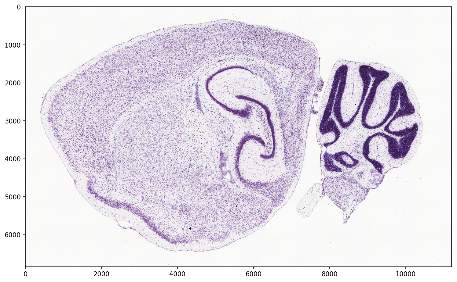
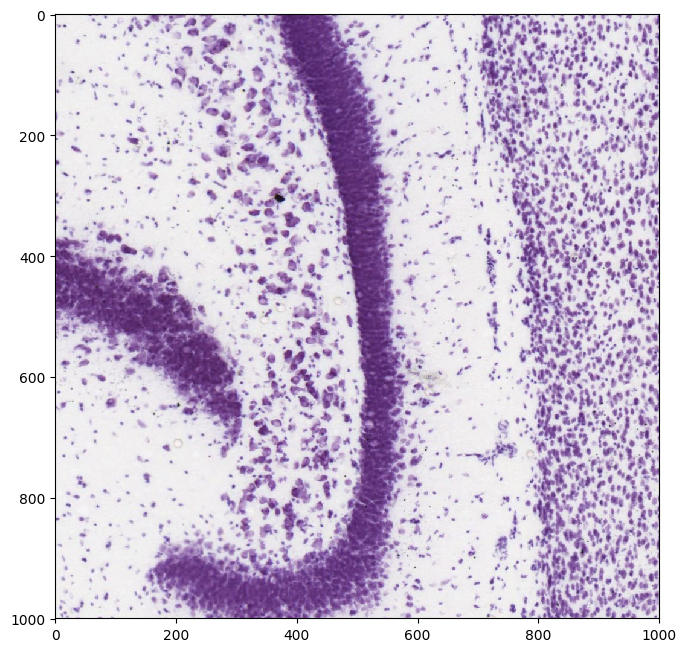
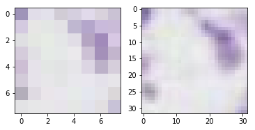
Let’s take a look at a portion of the image at various magnifications.

plt.figure(num=None, figsize=(8, 8), dpi=100, facecolor='w', edgecolor='k')
plt.imshow(np.uint8(img[3000:4000,6000:7000]))

plt.figure(num=None, figsize=(8, 8), dpi=100, facecolor='w', edgecolor='k')
plt.imshow(np.uint8(img[3250:3750,6250:6750]))

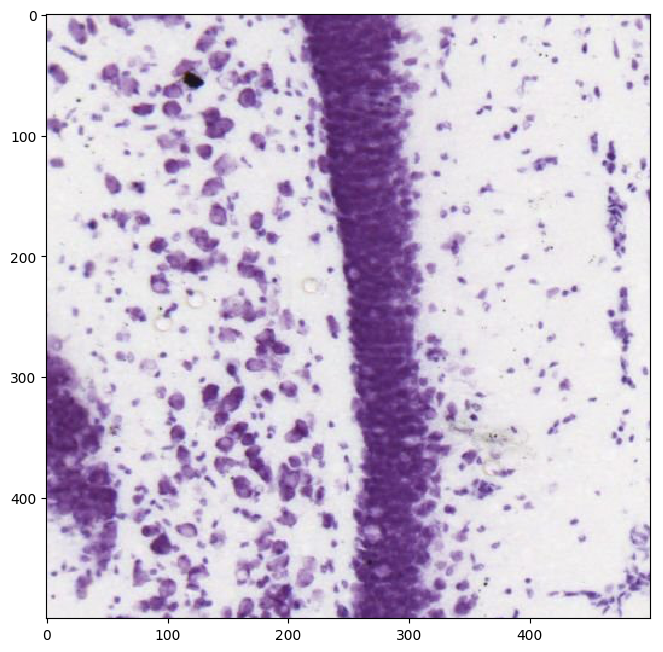
Looks like we have some fairly high-resolution images that allow us to make out the shapes and distinctions between the somas of various neurons. If we had a lower-resolution dataset or perhaps a dataset with more noise we might want to be able to apply a model to improve its resolution to be on par with what is shown above.

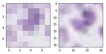
Generating examples

Next we’ll proceed with turning raw data into examples we can use for training. This will make use of a problem definition I recently contributed to the tensor2tensor data_generators which you can check out here.

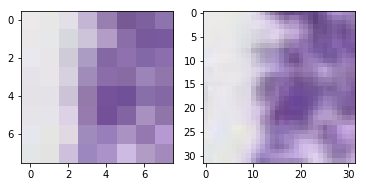
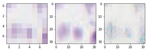
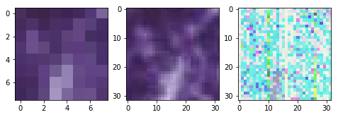
Our neural network will attempt to learn a mapping between an input image and a target image. The problem we’ll be working with takes the raw image and splits it up into 32px by 32px sub-images - we’ll use these as our targets. We’ll also use a down-sampled 8px by 8px version of these as our inputs.

In the following we’ll import that and call the generate_data method, providing the appropriate tmp and data dir paths (the former being the directory to which raw data will be downloaded and the latter being the directory to which TFRecord training examples will be generated).

from tensor2tensor.data_generators.allen_brain import Img2imgAllenBrainDim8to32

data_dir = "/mnt/nfs-east1-d/data"
tmp_dir = "/mnt/nfs-east1-d/tmp"

problem_object = Img2imgAllenBrainDim8to32()

problem_object.generate_data(data_dir, tmp_dir)

That will take at least an hour or so, depending on the speed of your internet connection. Once it’s finished you’ll be able to iterate over examples using tf.eager:

demo.show_random_examples(problem_object, data_dir, num=4)

Training the stock model

Let’s start by training the stock Tensor2Tensor Image Transformer model. Check out the paper here.

We’ll be using an early (unsupported) draft of a library I built to simplify the process of configuring and launching training jobs on Kubernetes + Kubeflow. In the somewhat near future it looks like this purpose will be well served by @wbuchwalter’s Faring which should be generalized beyond TensorFlow and provide more robust support for various interesting hyperparameter tuning strategies.

Training

Great now let’s do a long run on a node with multiple GPUs and a model of reasonable size.

args = _configure_experiment("allen-ngpu8",
                             problem="img2img_allen_brain_dim8to32",
                             num_gpu_per_worker=8,
                             hparams_set="img2img_transformer2d_tiny",
                             model="img2img_transformer",
                             extra_hparams={
                               "batch_size": 18,
                             },
                             num_steps=15000)

job = experiment.T2TExperiment(**args)
job.run()

experiment_data = demo.event_data_for_comparison("gs://kubeflow-rl-checkpoints/comparisons/allen-ngpu8*")
demo.show_experiment_loss(experiment_data)

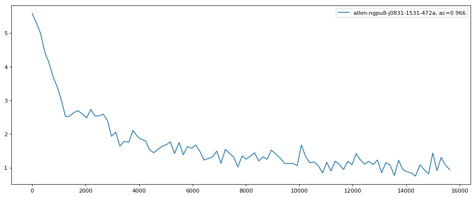
Our model does not seem to converge smoothly but rather continues to vary significantly. This could be due to using an overly-small batch size. While this is the largest batch size that was able to train on our current hardware (an NVIDIA K80 GPU), we might try distributing over multiple machines with 8x GPUs thereby increasing the effective batch size by the multiplicity of that distribution.

We might also consider using a different architecture that scales in image size more efficiently than the Image Transformer model (I believe such as the U-Net).

Qualitative analysis

Now that our model is trained we can take a look at its predictions and see how well it’s doing and how it might be improved. Imaging problems are great in this regard because we can visually see where the problem is under-performing to gain insight into how to improve it. This is true of other modalities but harder with those that can’t be readily visualized like high-dimensional non-visual time-series data.

from tensor2tensor.utils import trainer_lib
from tensor2tensor import problems
from tensor2tensor.utils import registry
import tensorflow as tf
Modes = tf.estimator.ModeKeys

hparams_set = "img2img_transformer2d_tiny"
problem_name = "img2img_allen_brain_dim8to32"
model_name = "img2img_transformer"
data_dir = "/mnt/nfs-east1-d/data"

hp = trainer_lib.create_hparams(
    hparams_set,
    data_dir=data_dir,
    problem_name=problem_name)

model = registry.model(model_name)(hp, Modes.TRAIN)

problem_object = problems.problem(problem_name)

dataset = problem_object.dataset(Modes.TRAIN, data_dir)

ckpt_path = "gs://kubeflow-rl-checkpoints/comparisons/allen-ngpu8/allen-ngpu8-j0831-1531-472a/model.ckpt-4586"

_ = demo.predict_ith(1234, ckpt_path, dataset, model)

_ = demo.predict_ith(1234, ckpt_path, dataset, model)

_ = demo.predict_ith(1234, ckpt_path, dataset, model)

_ = demo.predict_ith(1234, ckpt_path, dataset, model)

_ = demo.predict_ith(1234, ckpt_path, dataset, model)

_ = demo.predict_ith(1234, ckpt_path, dataset, model)

_ = demo.predict_ith(1234, ckpt_path, dataset, model)

_ = demo.predict_ith(1234, ckpt_path, dataset, model)

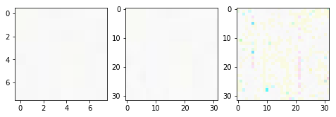
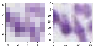
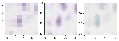
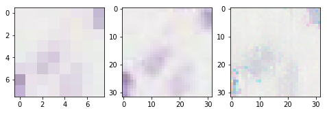
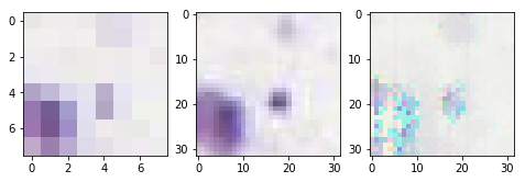
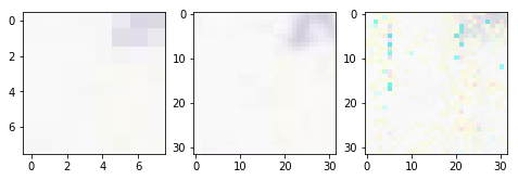
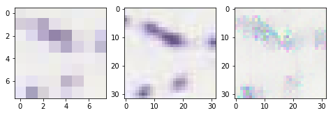
Interesting. First of all, in many cases our model does seem to be inferring something of higher-resolution from the lower-resolution input that looks approximately correct in some sense. But with the presence of distinctly pink and teal pixels. It seems the second example above is an extreme case of this and in general it tends to happen in the darker portions of the image.

Additionally there appear to be vertical streaks in regular positions across all of the examples.

There are multiple directions to go from here.

Larger model

First of all, the model we used for this problem was very small, coming from the img2img_transformer_tiny hparam set, which seems to be primarily meant for testing and debugging. Here’s its specification:

def img2img_transformer_tiny():
  """Tiny params."""
  hparams = img2img_transformer2d_base()
  hparams.num_hidden_layers = 2
  hparams.hidden_size = 128
  hparams.batch_size = 4
  hparams.max_length = 128
  hparams.attention_key_channels = hparams.attention_value_channels = 0
  hparams.filter_size = 128
  hparams.num_heads = 1
  hparams.pos = "timing"
  return hparams

In contrast, for example, img2img_transformer2d_n24 uses the following:

def img2img_transformer2d_n24():
  """Set of hyperparameters."""
  hparams = img2img_transformer2d_base()
  hparams.batch_size = 1
  hparams.hidden_size = 1024
  hparams.filter_size = 2048
  hparams.layer_prepostprocess_dropout = 0.2
  hparams.num_decoder_layers = 8
  hparams.query_shape = (8, 16)
  hparams.memory_flange = (8, 32)
  return hparams

Normalization

We should probably normalize our examples to have zero norm and unit variance. This should be done using the mean and variance of the dataset as a whole which can be approximated using a random sample of sub-images across different slices. Currently examples come directly from the Allen Inst. API which serves images which are of course not normalized.

Better loss function

We might also explore adding an adversarial loss. The above visual features are quite obvious for us to detect - simply being the presence of pixels of particular colors or the presence of distinct visual lines. It is reasonable to expect that a discriminator network could learn to detect these features. In doing so it would be interesting to extend the existing loss, which seems to perform reasonably well, with the adversarial loss (i.e. use a hybrid).

Smaller up-sampling ratio

We might explore a smaller up-sampling ratio. In this case, this ratio (from 8px by 8px to 32px by 32px) is 4x. Perhaps we could either consider only an up-sampling ratio of 1.25x or consider a schedule of increasing this ratio throughout training.

Larger effective batch size

As mentioned above, one direction going forward would be to distribute training over multiple 8x GPU machines, thereby increasing the effective batch size (and presumably the smoothness of the optimization) even further. Increasing the batch size of course doesn’t always lead to improvements in performance but in this case our effective batch size is still rather small - 18*8 = 144.

With that said, the pix2pix work by Isola et al. (2017) used a batch size of only 10 when comparing with an encoder-decoder architecture. Either a small batch size may be sufficient in the case of our current architecture or a change in architecture might permit a reduction in batch size.

Consider a different architecture

More generally than in regard to the batch size question - Isola et al. (2017) have reported good results using U-Nets for hybrid-loss adversarial image translation, e.g. pix2pix with patch sizes up to 284x284 on a Titan X GPU (12GB memory). Such an approach would also be worth exploring for the sake of comparison.

Simplify the problem

We could try simplifying the problem by converting these images to greyscale. Although the stain we’re using has a purple color, it is in effect a binary indicator.

To be continued…

That’s all for Part I of our continuing series. Stay tuned next week when see how the above improves with normalization and perhaps an alternative loss or architecture.